Examples of pseudospectra
See also Examples from engineering, and the

Three examples are shown here:
Here is an
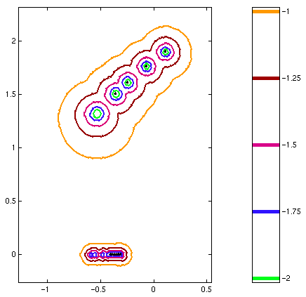
example of a matrix (the reaction-diffusion
Brusselator model of dimension 800, taken from Matrix Market) where the
computation indicates that non-normality is not significant. The
smallest epsilon-pseudospectrum shown is 10-2 and the scale
of the entire picture is O(1). The diameter of the
10-2-pseudospectrum is not much bigger than
2*10-2, which shows that the matrix is reasonably normal
and that the Ritz values returned should be both accurate and
physically meaningful. 
This
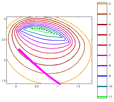
example is very different to the above. The matrix is the `Grcar
matrix' of dimension 400, and the smallest epsilon-pseudospectrum
shown is 10-11 even though the axis scale is
O(1). This indicates that this matrix is strongly
non-normal. The eigenvalues returned by the Arnoldi iteration are
shown as black dots. The actual eigenvalues of the matrix are
shown as magenta stars. They lie nowhere near the Arnoldi values. This
is a typical example of what can happen when computing eigenvalues of
a very non-normal matrix. The Arnoldi iteration has converged to
eigenvalues of a slightly perturbed matrix, but in this case the
non-normality is so extreme that these are far from
the true eigenvalues. 
Perhaps
the most important situation is where machine precision is sufficient
to converge to eigenvalue estimates, but pronounced non-normality may
nevertheless diminish the physical significance of some of them. An
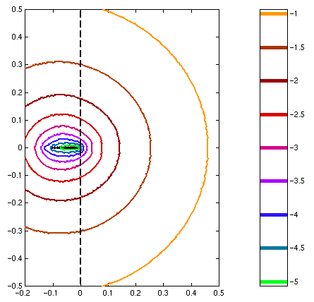
example of a case in which this is important is the matrix created by
linearisation about the laminar solution of the Navier-Stokes
equations for fluid flow in an infinite circular pipe. (Our matrix is
obtained by a Petrov-Galerkin spectral discretisation of the
Navier-Stokes problem due to Meseguer and Trefethen. The axial and
azimuthal wave numbers are 0 and 1, respectively.) The pseudospectra
are shown below, and although the eigenvalues all have negative real
part, implying stability of the flow, the pseudospectra protrude far
into the right half-plane. This implies pronounced transient growth of
some perturbations of the velocity field in the pipe, which in the
presence of nonlinearities in practice may lead to transition to
turbulence. 
Pseudospectra GUI home page.
|


