Projection Tutorial

This tutorial is designed to take you through an example where the the time needed to create a high-resolution publication quality plot of the pseudospectra of a matrix is significantly reduced by projection onto a carefully chosen invariant subspace.

You must have the Pseudospectra GUI installed on your machine to be able to work through this tutorial. You can download it by clicking here.

The tutorial is organised into five parts:

• Step 1: Set up the data
• Step 2: Select the portion of the complex plane of interest
• Step 3: Begin to introduce projection
• Step 4: Reduce the Safety value still further
• Step 5: Compute the pseudospectra on a fine grid of size 200 by 200

You can download the code used to generate the matrices used in this tutorial by clicking here. This is taken from Trefethen's paper, Computation of Pseudospectra (Acta Numerica, 1999), which describes projection in greater detail.

• Step 1: Set up the data.

  Generate the matrix B by downloading the code and running it with N=200:

  B = lnt_comp_psa_mtxs(200);

  Compute the pseudospectra using the default settings:

  psa(B)

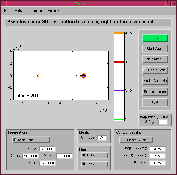
  You should end up with something like the following image, which takes about 30 seconds to generate on my Sun Ultra 5 workstation.

  Note the large magnitudes of the x and y axes. Thes axes are chosen automatically by the Pseudospectra GUI, and are this big because of the outlying eigenvalue near -80,000.

  

Pseudospectra GUI home page.